Machine Learning Made Easy

Simple Linear Regression

Assume we have $n$ pieces of input data — or "samples" — each represented by $x_i$ where $i = [1 ... n]$. Likewise assume we have $n$ pieces of corresponding output data — or "observations" — each represented by $y_i$.

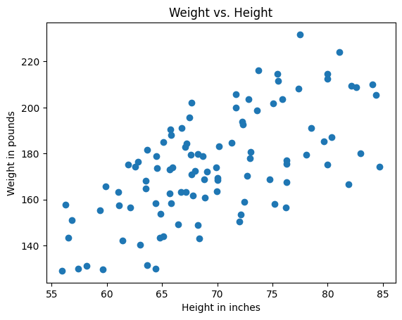
For this exercise, we will simulate data measuring the height and weight of a random population.

import numpy as np
import matplotlib.pyplot as plt

NUM_SAMPLES = 100
rng = np.random.default_rng()

heights = np.linspace(60, 80, NUM_SAMPLES) * rng.uniform(0.9, 1.1, NUM_SAMPLES)
weights = heights * rng.uniform(2, 3, NUM_SAMPLES)

def make_plot():
    _, ax = plt.subplots()
    ax.set_xlabel("Height in inches")
    ax.set_ylabel("Weight in pounds")
    ax.set_title("Weight vs. Height")
    return ax

ax = make_plot()
ax.scatter(heights, weights)
plt.show()

Linear Regression

A function that takes a sample and predicts the corresponding observation is called a "model." If we drew a "line of best fit" through the middle of the points in our scatterplot, we would have a working model: we could take any height $x_i$, find the corresponding point $(x_i, \hat y_i)$ on our line, and take the $\hat y_i$ value as our predicted weight. This is the basic idea behind "linear regression."

We can represent our line as:

$$ \hat y_i = a x_i + b $$

Here $ \hat y_i $ ("y hat i") indicates a prediction, while $y_i$ indicates an observation.

The key is picking the best possible values for $a$ and $b$. We can think of this as a minimization problem: using predictions will inevitably cause some loss in accuracy vs. observations. Our goal is to minimize that loss.

Loss

To minimize loss, we first need to represent our loss with a "loss function" $L$ that is differentiable. If we can take the derivative of $L$, we can find the minimum by solving for $a$ and $b$ when $L' = 0$.

We can take the difference $y_i - \hat y_i$ to measure the inaccuracy or "residual" in our model for $x_i$. We want to add all of these residuals together to measure the total loss, and we need to keep these residuals positive to avoid negative values "cancelling out" positive values and making the loss look lower than it really is. Squaring a number makes it positive, and finding the derivative of $x^2$ is trivial, so we will square the residuals like $(y_i - \hat y_i)^2$.

If we sum up the residuals for every piece of data this way, we have a loss function known as the "residual sum of squares:"

$$ L = \sum (y_i - \hat y_i)^2 $$

Replacing $ \hat y_i $ with the equation for our line yields:

$$ L = \sum (y_i - a x_i - b)^2 $$

Now we can find the values for $a$ and $b$ that minimize $L$.

Minimizing Loss

We minimize loss by finding two partial derivatives of $L$: one with respect to $a$ and the other with respect to $b$. Each partial derivative represents the rate of change in $L$ caused by a change in the corresponding parameter $a$ or $b$. When that rate of change hits zero, we know we've found the value for that parameter which minimizes its contribution to $L$.

Partial derivative with respect to $a$:

$$ \frac{\partial L}{\partial a} = (2) \sum (y_i - a x_i - b) (-x_i) $$

Set to $0$ and simplify:

$$ \begin{alignedat}{1} 0 & = (2) \sum (y_i - a x_i - b) (-x_i) \\ 0 & = (2) \sum (y_i - a x_i - b) (-1) (x_i) \\ 0 & = \sum (y_i - a x_i - b) (x_i) \\ 0 & = \sum (x_i y_i - a x^2_i - b x_i) \\ 0 & = \sum x_i y_i - a \sum x^2_i - b \sum x_i \\ \sum x_i y_i & = a \sum x^2_i + b \sum x_i \end{alignedat} $$

Partial derivative with respect to $b$:

$$ \frac{\partial L}{\partial b} = (2) \sum (y_i - a x_i - b) (-1) $$

Set to $0$ and simplify:

$$ \begin{alignedat}{1} 0 & = (2) \sum (y_i - a x_i - b) (-1) \\ 0 & = \sum (y_i - a x_i - b) \\ 0 & = \sum y_i - a \sum x_i - b n \\ \sum y_i & = a \sum x_i + b n \end{alignedat} $$

To make algebraic manipulation easier, let:

$$ \begin{alignedat}{1} C & = \sum x_i y_i \\ D & = \sum x_i^2 \\ E & = \sum x_i \\ F & = \sum y_i \end{alignedat} $$

Then we can make the following simplification:

$$ \begin{alignedat}{1} \sum x_i y_i &= a \sum x^2_i + b \sum x_i \\ C &= aD + bE \end{alignedat} $$

As well as:

$$ \begin{alignedat}{1} \sum y_i &= a \sum x_i + b n \\ F &= aE + bn \end{alignedat} $$

Solution

We now have two equations with two unknowns: $a$ and $b$. We can solve for the unknowns by taking the difference of the equations. First scale the equations to make it easy to eliminate the $b$ term and find $a$:

$$ \begin{alignedat}{1} (aE + bn = F)E & \Rightarrow aE^2 + bnE = EF \\ (aD + bE = C)n & \Rightarrow anD + bnE = nC \end{alignedat} $$

Then subtract:

$$ \begin{alignedat}{1} aE^2 + bnE &= EF \\ -(anD + bnE &= nC) \\ \hline aE^2 - anD &= EF - nC \end{alignedat} $$

And rearrange: $$ \begin{alignedat}{1} a(E^2 - nD) &= EF - nC \\ a &= \frac{EF - nC}{E^2 - nD} \end{alignedat} $$

Do likewise to find $b$:

$$ \begin{alignedat}{1} (aD + bE = C)E &\Rightarrow aDE + bE^2 = CE \\ (aE + bn = F)D &\Rightarrow aDE + bnD = DF \end{alignedat} $$

Subtract: $$ \begin{alignedat}{1} aDE + bE^2 &= CE \\ -(aDE + bnD &= DF) \\ \hline bE^2 - bnD &= CE - DF \end{alignedat} $$

Rearrange:

$$ \begin{alignedat}{1} b(E^2 - nD) &= CE - DF \\ b &= \frac{CE - DF}{E^2 - nD} \end{alignedat} $$

Note that we took care to give $a$ and $b$ a common denominator. In code, we will be able to calculate that denominator once and reuse it. If you do not follow this exact procedure (many others will work), the denominators might not initially be the same — this is easily fixed by multiplying one of the fractions by $ \frac{-1}{-1} $.

Expanding with our substitutions yields:

$$ \begin{alignedat}{1} a &= \frac{\sum x_i \sum y_i - n \sum x_i y_i}{(\sum x_i)^2 - n\sum x_i^2} \\ b &= \frac{\sum x_i y_i \sum x_i - \sum x_i^2 \sum y_i}{(\sum x_i)^2 - n\sum x_i^2} \end{alignedat} $$

This is a general solution for Simple Linear Regression — "simple" because we are working with a single variable (height) for each piece of input data.

Basic Implementation

Now we can build our line of best fit and plot it against our data.

C = heights.dot(weights)
D = heights.dot(heights)
E = heights.sum()
F = weights.sum()
denominator = E**2 - NUM_SAMPLES*D

a = (E*F - NUM_SAMPLES*C) / denominator
b = (C*E - D*F) / denominator
predicted_weights = a*heights + b

ax = make_plot()
ax.scatter(heights, weights)
ax.plot(heights, predicted_weights)
plt.show()

Building a Reusable Model

Now that we understand how simple linear regression works, we can easily create a reusable model that can be applied to any suitable data set.

First, we write the data structure which represents the model:

from dataclasses import dataclass

@dataclass
class Model:
    a: float = 0.0
    b: float = 0.0

Next, we write a function that takes input data (arrays of samples and observations) and returns a model:

def make_model(samples: np.ndarray, observations: np.ndarray) -> Model:
    n = samples.shape[0]
    c = samples.dot(observations)
    d = samples.dot(samples)
    e = samples.sum()
    f = observations.sum()
    denominator = e**2 - n*d

    model = Model()
    model.a = (e*f - n*c) / denominator
    model.b = (c*e - d*f) / denominator

    return model

Finally, we write a function that takes as input a model and an array of samples, and returns an array of corresponding predictions:

def predict(model: Model, samples):
    result = model.a*samples + model.b
    return result

We can now use these general purpose facilities to create a model based on our sample data:

model = make_model(heights, weights)

And then we can create a series of predicted observations using that model:

predicted_weights = predict(model, heights)

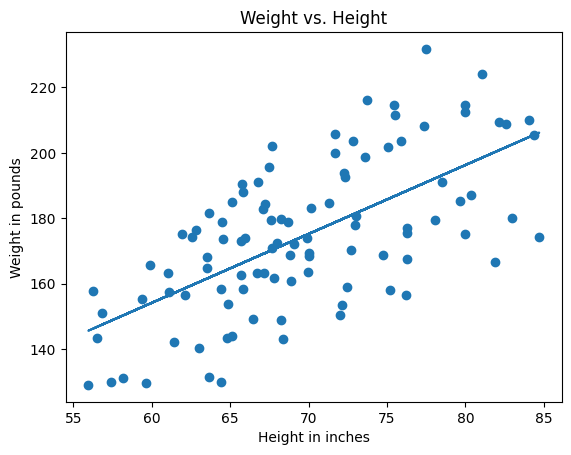
Plotting our predicted weights against the actual weights yields the following:

ax = make_plot()
ax.scatter(heights, weights)
ax.plot(heights, predicted_weights)
plt.show()

Assessing Model Performance

How well does our model work? One useful way to answer that question is by calculating the coefficient of determination, or "R squared:"

$$ R^2 = 1 - \frac{SS_{res}}{SS_{tot}} $$

Where $ {SS}_{res} $ is the residual sum of squares:

$$ {SS}_{res} = \sum(y_i - \hat{y}_i)^2 $$

And $ {SS}_{tot} $ is the total sum of squares:

$$ {SS}_{tot} = \sum(y_i - \bar{y})^2 $$

Here $ \bar{y} $ ("y bar") denotes the mean observation, which is the average actual weight in our scenario.

def get_r2(observations, predictions) -> float:
    ss_res = np.sum((observations - predictions)**2)
    ss_tot = np.sum((observations - observations.mean())**2)
    r2 = 1 - ss_res / ss_tot
    return r2

r2 = get_r2(weights, predicted_weights)

from IPython import display
display.display_markdown(f"$$ R^2 = {r2:.2} $$", raw=True)

$$ R^2 = 0.42 $$

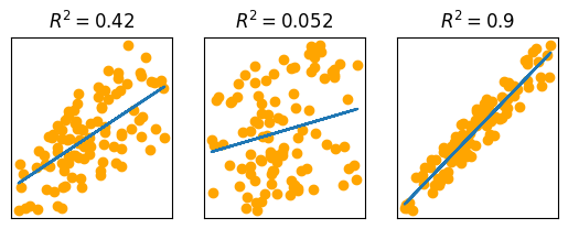
Intuitively, a higher $ R^2 $ indicates better model performance. We can observe this by comparing $ R^2 $ values for data with a wider or tighter spread of sampled weights:

weights_wide = heights * rng.uniform(1, 4, NUM_SAMPLES)
model_wide = make_model(heights, weights_wide)
predicted_weights_wide = predict(model_wide, heights)
r2_wide = get_r2(weights_wide, predicted_weights_wide)

weights_tight = heights * rng.uniform(2.3, 2.6, NUM_SAMPLES)
model_tight = make_model(heights, weights_tight)
predicted_weights_tight = predict(model_tight, heights)
r2_tight = get_r2(weights_tight, predicted_weights_tight)

_, axes = plt.subplots(1, 3, figsize=(6.4, 2.13))

for ax in axes:
    ax.set_xticks([])
    ax.set_yticks([])

axes[0].scatter(heights, weights, color='orange')
axes[0].plot(heights, predicted_weights)
axes[0].set_title(f"$ R^2 = {r2:.2} $")

axes[1].scatter(heights, weights_wide, color='orange')
axes[1].plot(heights, predicted_weights_wide)
axes[1].set_title(f"$ R^2 = {r2_wide:.2} $")

axes[2].scatter(heights, weights_tight, color='orange')
axes[2].plot(heights, predicted_weights_tight)
axes[2].set_title(f"$ R^2 = {r2_tight:.2} $")

plt.show()